Dynamic Identification of Serial Manipulators
Over the Summer of 2025, I had the opportunity to assist Chinmay Devmalya in the development of a new lightweight and compact robot arm called Maestro. I developed an optimization-based workflow for identifying the kinematic and inertial parameters of the robot once it is first assembled. The full project description is below.
Introduction
In order to precisely control the position and applied force at the end-effector of a serial manipulator, we need a precise geometric and inertial model of our manipulator. At design time, the dimensions of each link can be specified and inertial parameters of each link can be estimated using CAD software such as Fusion, Solidworks, or OnShape. However, these modeled geometric and inertial parameters rarely match exactly with those of the fully assembled robots. Common sources of this mismatch are tolerance stack up in machined parts or errors in component mass estimates. Rather than enforce tighter (unrealistic) tolerances on machined parts or weigh each individual component before assembly to improve the accuracy of our model, we can use data-driven methods to estimate the geometric and inertial parameters of using motion data collected from the real robot.
Here we outline methods to identify the geometric and dynamic parameters of our manipulator using symbolic libraries and numerical optimization
Kinematic Identification Principles
When identifying the kinematic properties of our robot, we wish to identify the link lengths of each joint.
\[\begin{matrix} p \in\mathbb{R}^3 \text{- Joint Origin} \\ o \in SO^3 \text{- Joint Orientation} \\ r \in\mathbb{R}^3 \text{- Joint Axis} \end{matrix}\]We represent the collection of all kinematic variables $(p_0, o_0, r_0, \ldots, p_N, o_N, r_N)$.
Let us define the pose of the end-effector as $z\in \mathbb{R}^6$ and a forward kinematics function $f$
\[z=f(q, \Gamma)\]Depending on the geometry of the manipulator, the function $f$ can be nonlinear.
We can identify the robot kinematically by sampling $N$ joint space positions, measuring the end-effector position, and solving the following nonlinear optimization. Here we use IPOPT to solve the problem.
\[\Gamma^* = \arg\min_{\Gamma}\Sigma_{i}\|z^i-f(q^i, \Gamma)\|_2\]Dynamic Identification Principles
When identifying the dynamic parameters of the manipulator, we would like to identify the following inertial parameters for each link.
\[\begin{matrix} m_i\text{ - Mass of link $i$} \\ l_i\text{ - Lever of link $i$} \\ I_i\text{ - Inertia Matrix of link $i$}\\ \end{matrix}\]Because these parameters have physical significance, they can only take on physically realizable values. $m_i$ must be a positive number and $I_i$ must be a positive-definite matrix. We represent the collection of all inertial variables $(m_0, l_0, I_0,\ldots, m_N, l_N, I_N)$ with the symbol $\Theta$.
Given the joint positions, velocities, and accelerations of our robot there exists a linear relationship between our inertial parameters and our joint torques
\[\begin{matrix} \tau=Y(q, \dot{q}, \ddot{q})\Theta \end{matrix}\]Sources of Error in Y
In an ideal world with a perfectly rigid manipulator, and perfect torque sensing, our $Y$ would be perfectly accurate. However, due to things such as sensor noise and un-modeled dynamics, our torque observations can be noisy. We can consider our joint torques to be a random variable sampled from the following gaussian distribution
\[\tau\sim\mathcal{N}(Y(q, \dot{q}, \ddot{q})\Theta, \Sigma)\]Where $\Sigma$ is the covariance matrix of our random variable.
Information in Identification
When identifying a manipulator, we sample data from our robot to define a linear least squares problem of the following form
\[\arg\min_x\|Ax - b\|\]The regressor matrix $A$ is determined by the choice of $q$ in the case of kinematic identification, and $q, \dot{q}, \ddot{q}$ in the case of dynamic identification. In both cases, we would like to ensure that our observations $b$, make our underlying parameters as clear as possible.
One way to quantify this “clearness” is thinking about the derivative of our observations with respect to our parameters. If the derivative of our observation with respect to our parameters is small, we will struggle to differentiate between changes in observation caused by sensor noise and changes caused by parameter mismatch. However, if our derivative with respect to parameters is large, this distinction is much easier to make. In our case, this derivative is our $A$ matrix.
\(\frac{\partial b^*}{\partial x} = A\) We can express the magnitude of a matrix as a scalar using the following
\[\det(A^TA)\]In the case that our observation $b$ has uniform covariance, the above scalar is a sufficient metric for the robustness of our regressor matrix. However, in the case of non-uniform observation covariance, we would like to minimize our dependence on observation vectors in noisy directions and maximize our dependence on observation vectors in less noisy directions. An updated metric that captures this is the following
\[\det(A^T\Sigma^{-1}A)\]This is the determinant of the Fisher Information matrix $\mathcal{I}$
\[\begin{matrix} \mathcal{I}=A^T\Sigma^{-1}A\\ \det(A^T\Sigma^{-1}A) = \det(\mathcal{I}) \end{matrix}\]Optimizing Trajectory for Dynamic ID
When choosing a dynamic trajectory, we need to choose a series of $q, \dot{q}, \ddot{q}$ that optimizes the robustness metric we discussed above. Rather than choosing each of these values individually, which could lead to infeasible trajectories, we instead parameterize our joint trajectories using a sum of sinusoidal functions adopted from (3).
\[\begin{matrix} q_i(t)=\sum_{l=1}^N\frac{a^{i}_l}{w_fl}\sin(w_flt)-\frac{b^{i}}{w_fl}\cos(w_flt) + q_{i0} \\ \dot{q}_i(t)=\sum_{l=1}^N a^{i}_l\cos(w_flt)+b^{i}_{l}\cos(w_flt)\\ \ddot{q}_i(t)=\sum_{l=1}^N -a^{i}_lw_fl\sin(w_flt)+b^{i}_l{w_fl}\cos(w_flt)\\ \end{matrix}\]Now, rather than choosing each $q, \dot{q}, \ddot{q}$, we instead choose $a^i, b^i, q_0^i$ for each joint $i$ in our manipulator. Our sinusoidal parameters can be represented using the following matrices
\[\begin{matrix} A :=\begin{bmatrix} a^{0}_{0} & a^{1}_{0} & \cdots & a^{M}_0 \\ a^{0}_{1} & a^{1}_{1} & \cdots & a^{M}_1 \\ \vdots & \vdots & \cdots & \vdots \\ a^{0}_{N} & a^{1}_{N} & \cdots & a^{M}_{N} \end{bmatrix}, \qquad B := \begin{bmatrix} b^{0}_{0} & b^{1}_{0} & \cdots & b^{M}_0 \\ b^{0}_{1} & b^{1}_{1} & \cdots & b^{M}_1 \\ \vdots & \vdots & \cdots & \vdots \\ b^{0}_{N} & b^{1}_{N} & \cdots & b^{M}_{N} \end{bmatrix}\\\\ \end{matrix}\]Collision Avoidance
During an identification trajectory we must ensure that the robot does not collide with itself or with the ground plane that supports it. There are two reasons for this: the first is safety as collisions can damage the robot, the second is that when the robot has a collision the object the robot collides with imparts an un-modeled torque on the actuators which complicates identification.
Quick and Dirty Solution: Joint-Space constraints
A simple solution reduce the change of collisions is to adjust the joint limits $q_\text{low}, q_\text{high}$ of our optimization such that self-collisions due to individual joints are not possible. For example, when running this optimization on Maestro, the joint limits for joints 6 and 7 needed to be adjusted to avoid collisions.
In addition to preventing self-collisions, we must make sure that the end-effector of the robot stays above the ground-plane. We can include a forward-kinematics calculation within our optimization and add a constraint that the z-height of the end-effector stays above 0.
Though these do not prevent all possible collisions, such as the end-effector with other points of the robot however, we can prune and eliminate any such trajectories before running on on the real robot.
Trajectory Optimization Problem
We can now create the following optimization problem to find our desired trajectory
\[\begin{align*} \arg\max_{A, B, q_0} \det(\bar{Y}^T\Sigma^{-1}\bar{Y}) \\\\ |A_{i,j}|\le a_\max \quad\forall i,j\\ |B_{i,j}|\le a_\max \quad\forall i,j\\ q_{\text{low}}\le q_t \le q_{\text{high}}\quad\forall t\\\\ f(q_t)\ge x_\text{floor}\quad\forall t\\ \dot{q}_0=\ddot{q}_0=0 \\ \dot{q}_{t_F}=\ddot{q}_{t_F}=0 \\ \end{align*}\]Solving for Dynamic Parameters
Given the regression matrix $\bar{Y}$, a reasonable way to identify our estimate $\hat{\Theta}$ would be to solve the following generalized least squares problem
\[\hat\Theta=\arg\min_{\hat{\Theta}}\quad(\bar{Y}\hat{\Theta} - \mathcal{T})^T\Sigma^{-1}(\bar{Y}\hat{\Theta} - \mathcal{T})\]where $\Sigma$ is the covariance of our torque observations. However, because $\bar Y$ is not full-rank, there may be an infinite number of possible solutions, not all of them physically valid. Two key conditions of physical validity for inertial are $m_i > 0$ and $I_i \succ 0$. To ensure that these conditions are met by our optimization we introduce the inertial variable formulation.
Inertia Variable Representation
Mass Representation
To ensure that our mass is always positive we can represent $m_i$ using the square of a number
\[m_i=z_i^2\]Where $z_i$ is the variable within our optimization problem associated with mass.
Inertia Matrix Representation
We represent the inertia matrix using a diagonalized Cholesky Decomposition that represents $I_i$ using a uni-triangular matrix $U_i$ and a diagonal matrix $D_i$. The full decomposition is shown below
\[I_i=U_iD_iU_i^T\]The collection of inertial variables representing the inertias of the manipulator $(z_0, l_0, U_0, D_0,\ldots,z_N, l_N, U_N, D_N)$ using the letter $\Psi$.
Constraints
In our optimization problem, we use constraints to encode the assumption that our initial estimate of the robot arm parameters is reasonable but needs some fine-tuning. Therefore, the majority of these constraints keep the iterate within some neighborhood of our original estimate.
Neighborhood Constraints
We define the neighborhood constraints for the parameters associated with each link here:
\[\begin{matrix} (z_i^2 - m_i^{0})^2 \le \alpha_i\\ \|l_i - l_i^0\|_2^2 \le \beta_i\\ \|u_i-u_i^0\|_2^2\le \gamma_i\\ \|d_i-d_i^0\|_2^2\le \delta_i\\ \end{matrix}\]where $\alpha, \beta, \gamma, \delta$ are scalar values that represent the limits from the initial estimate that we would like our result to stay within.
Cost
The reformulation of our inertial variables results in a nonlinear relationship between our inertial parameters and the torques of our system. We can re-write our cost as
\[\Sigma_i^T \|\tau^i - f(q^i, \dot q^i, \ddot q^i, \Psi)\|_{\Sigma^{-1}}\]Here $f$ is a multi-body inverse dynamics function such as the Reverse Newton Euler Algorithm.
Full Optimization
The full optimization problem is as follows
\[\begin{matrix} \arg\min_{\Psi}\quad\Sigma_i^T \|\tau^i - f(q^i, \dot q^i, \ddot q^i, \Psi)\|_{\Sigma^{-1}}\\ \text{s.t.}\\\\\ (z_i^2 - m_i^{0})^2 \le \alpha_i\\ \|l_i - l_i^0\|_2^2 \le \beta_i\\ \|u_i-u_i^0\|_2^2\le \gamma_i\\ \|d_i-d_i^0\|_2^2\le \delta_i\\ \end{matrix}\]Experiment Design
To evaluate our identification method, we can create a simulated robot to track our desired identification trajectory and use this to identify the robot. We then initialize our estimator with incorrect inertial estimates for multiple links and use our identification method to reduce the overall error.
Simulated Robot
We simulate our robot using Drake which contains tools both for multi-body simulation as well as joint-space control of our robot. To control our robot in simulation, we use Drake’s InverseDynamicsController which implements the following control law
\[\tau = -\tau_g(q)+m\left[\ddot{q}_d+K_p(q_d-q)+K_d(\dot{q}_d-\dot{q})\right]\]Our \(q_d, \dot{q}_d, \ddot{q}_d\) come directly from our optimized trajectory. After commanding our simulated robot to track our desired trajectory, we are left with $q_\text{exp}, \dot q_\text{exp}, \ddot q_\text{exp}$, our experimental joint positions, velocities, and accelerations. Combining this with our applied torque $\tau_\text{exp}$ we can create
Simulated Experiment
A video of the simulated experiment is shown below
Results
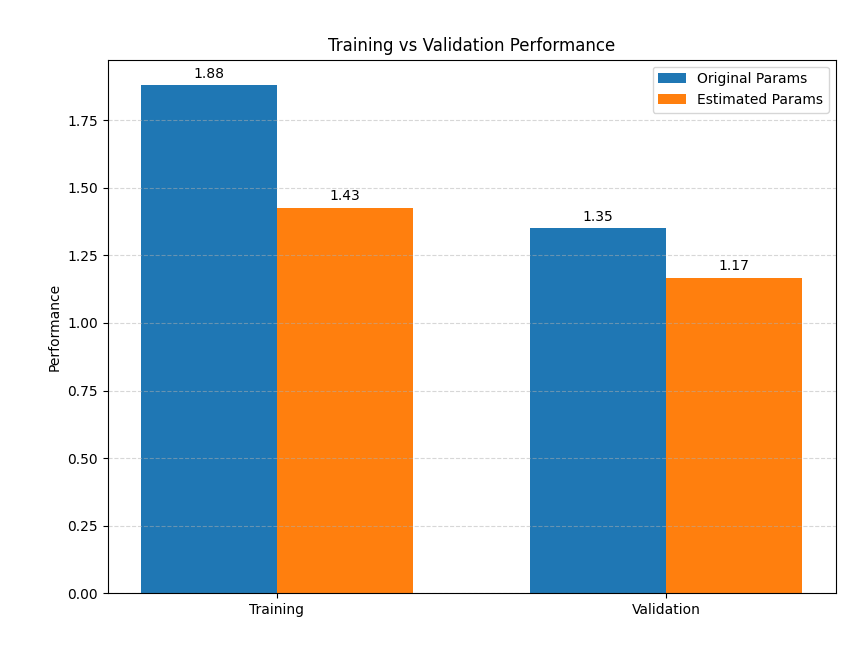
After solving our optimization problem to identify the inertial parameters using our experimental trajectory we then test the performance of our new, optimized parameters on an additional validation trajectory. Our evaluation metric is the same metric used within our parameter identification optimization.
\[L = \frac{1}{T}\Sigma_i^T \|\tau^i - f(q^i, \dot q^i, \ddot q^i, \Psi)\|_{\Sigma^{-1}}\]Below is a plot of the performance on the training and validation sets.
References
-
Excitation Trajectory Optimization for Dynamic Parameter Identification Using Virtual Constraints in Hands-on Robotic System - Tian et. al (linked here)
-
Optimal Excitation Trajectories for Mechanical Systems - Lee et. al (linked here)
-
Optimal Robot Excitation and Identification - Swevers et. al (linked here)
-
The Theory of Kinematic Parameter Identification for Industrial Robots - Everett, Hsu (linked here)
-
Identification of Fully Physical Consistent Inertial Parameters using Optimization on Manifolds - Traversaro et. al (linked here)