Nonlinear Bicycle Models for Vehicle Simulation
Introduction
Here, we will be walking through the modeling and simulation of a four-wheeled vehicle using a nonlinear bicycle model. The bicycle is a vehicle model that lumps each pair of front and rear wheels on a four-wheel vehicle into a single “virtual wheel” resulting in a two-wheeled virtual “bicycle”. A diagram of this model is shown below.
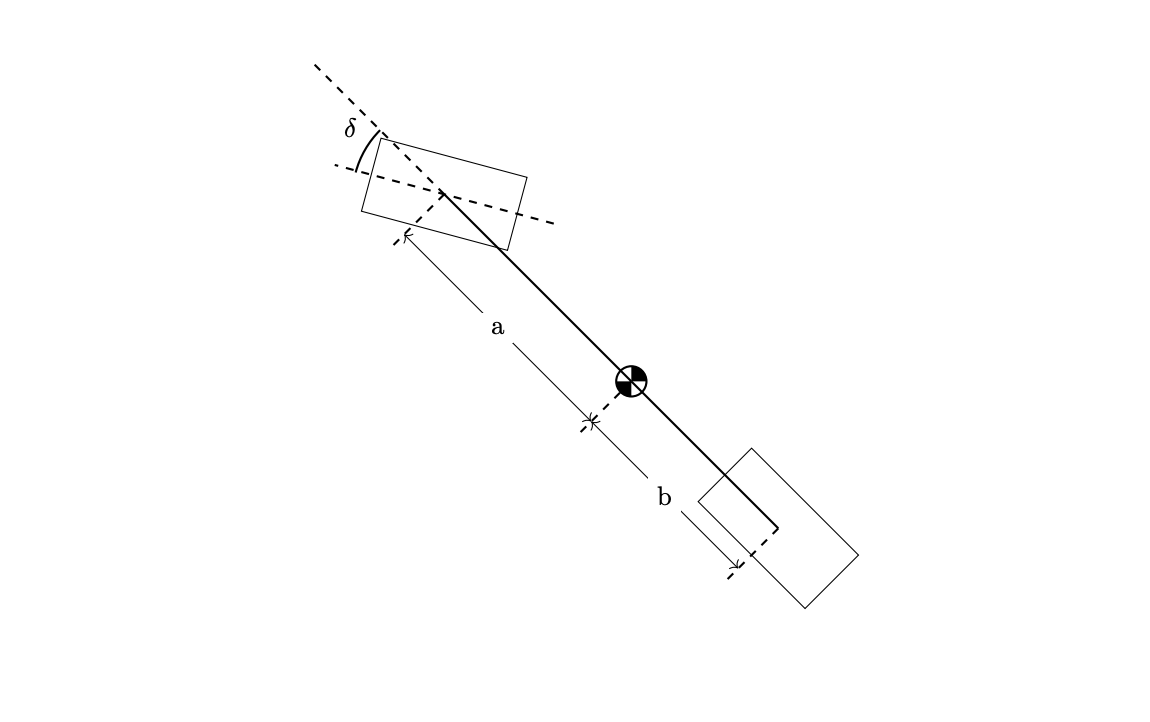
Despite this massive simplification, the bicycle model is still expressive enough to capture a large variety of drivetrains and vehicle engine locations such as front-wheel drive, rear-wheel drive, and mid-engined vehicles.
A key benefit of this model’s simplicity is that it is very computationally lightweight which means that it can be used within an optimization-based motion planner without much computational cost.
Vehicle Modeling
When modeling our vehicle, we will keep track of the following three state variables:
\[\begin{matrix} U_x \text{ - Vehicle Longitudinal Velocity}\\ U_y \text{ - Vehicle Lateral Velocity}\\ r \text{ - Vehicle Yaw rate (about CoM)} \end{matrix}\]Our goal is do develop a function that maps these vehicle state variables to vehicle state derivatives.
\[\left[\dot{U}_y, \dot{U}_x, \dot{r}\right]^T=f(U_x, U_y, r)\]There are two steps needed to arrive at this all-powerful $f(…)$ function: equations of motion and a model of our simulated tires.
Equations of Motion
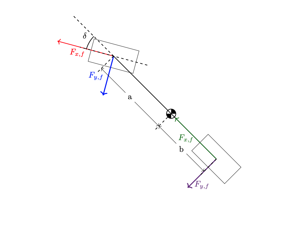
Our vehicle’s equations of motion assume that the only forces acting on the vehicle are imparted by its two tires. Each tire can impart a lateral and a longitudinal force $F_x$ and $F_y$ and summing the contribution of these forces gives us the next longitudinal, lateral, and rotational forces and moments $F_{\text{net}, x}$ , $F_{\text{net}, y}$, $\tau_\text{net}$.
\[\begin{matrix} F_{\text{net}, x} = F_{x_f}\cos{\delta} - F_{y_f}\sin{\delta} + U_yr \\ F_{\text{net}, y} = F_{x_f}\sin{\delta} + F_{y_f}\sin{\delta} - U_yr\\ \tau_{\text{net}} = \left[F_{x_f} \sin(\delta) + F_{y_f} \cos(\delta)\right] a - F_{y_r} b \\ \end{matrix}\]From here, it is straightforward to derive our vehicle accelerations by dividing by the vehicle mass and moment of inertia where appropriate to give us the following equations.
\[\begin{matrix} \dot{U}_x &= \frac{F_{x_f} \cos(\delta) - F_{y_f} \sin(\delta) + F_{x_r}}{m} + U_y r \\ \dot{U}_y &= \frac{F_{x_f} \sin(\delta) + F_{y_f} \cos(\delta) + F_{y_r}}{m} - U_x r \\ \dot{r} &= \frac{\left[F_{x_f} \sin(\delta) + F_{y_f} \cos(\delta)\right] a - F_{y_r} b}{I_{zz}} \end{matrix}\]Below is a python snippet of those same equations
ux_dot = (-fyf * np.sin(delta_f) + fxf * np.cos(delta_f) + fxr) / M - (r * uy)
uy_dot = (fyf * np.cos(delta_f) + fxf * np.sin(delta_f) + fyr) / M - (r * ux)

r_dot = (a * (fyf * np.cos(delta_f) + fxf * np.sin(delta_f)) - b * fyr)/ Izz
Tire Model
Now that we have the equations of motion, we can turn our focus to calculating the $F_x$ and $F_y$ of each tire. In this case, we will use the Fiala Tire Model which is simple but still captures tire grip limits. Though we have chosen the Fiala Model here, this is only one of many available tire models.
The longitudinal force, $F_x$ of each tire is treated as a control input while the lateral force of the tire, $F_y$ is determined by two variables the tire slip angle $\alpha$ and the tire’s cornering stiffness $C$.
The tire’s slip angle is the angle between its direction of travel and its orientation. A diagram demonstrating slip In our case, we can calculate slip angle as follows
\[\begin{matrix} \alpha_f = \text{atan2}(U_y + a\cdot r, U_x) - \delta \\ \alpha_r = \text{atan2}(U_y - b\cdot r, U_x) \end{matrix}\]The lateral force is determined by the below expression.
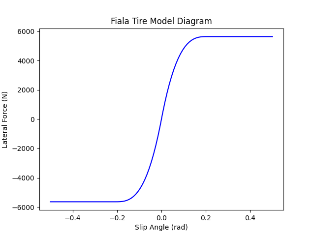
\[F_y = \begin{cases} F_{y,\text{Fiala}} = -C_\alpha \tan(\alpha) + \frac{C_\alpha^2 \tan(\alpha) |\tan(\alpha)|}{3 \mu F_z} - \frac{\left[C_\alpha \tan(\alpha)\right]^3}{27 (\mu F_z)^2}, & \left|F_{y,\text{Fiala}}\right| < \left|F_{y,\text{slip}}\right| \\ F_{y,\text{slip}} = -\mu F_z \, \text{sign}(\alpha), & \left|F_{y,\text{Fiala}}\right| \geq \left|F_{y,\text{slip}}\right| \end{cases}\]As we can see there are are actually two cases here. The first case is when the tire is when the tire is not slipping. At small slip angles, this curve is almost perfectly linear. As the tire slip angle increases, this the available tire lateral force becomes more and more nonlinear until it plateaus at $\mu F_z$.
If we think about our experience with tires in the real world this behavior makes sense. In a car we can corner harder and harder until our tires reach their limit and start sliding. This is usually accompanied by squealing and sometimes smoke. Below we can see a diagram of tire lateral forces with respect to slip angle for a Fiala tire model.
Full Python Implementation
Below is an implementation of the full bicycle model in Python.
import numpy as np
from scipy import constants

# Multiplier to convert forces from the order of 1e0 to
# the order of 1e3

FX_MULTIPLIER = 1e3

def slip_angles(veh_state, veh_ctrls, a_m, b_m):
    # Given vehicle state and controls
    # calculate slip angles front and rear

    ux, uy, r = veh_state[0], veh_state[1], veh_state[2]
    delta_f, fxf, fxr = veh_ctrls[0], veh_ctrls[1], veh_ctrls[2]

    alpha_f = np.arctan2(uy + a_m * r, ux) - delta_f
    alpha_r = np.arctan2(uy - b_m * r, ux)

    return alpha_f, alpha_r


def fiala_tire_np(alpha, f_x, f_z, mu, c_stiff):
	# Implementation of Fiala tire model
    fy_max = np.sqrt((mu * f_z) ** 2 - (f_x) ** 2)
    alpha_max = np.arctan2(3 * fy_max, c_stiff)
    tan_a = np.tan(alpha)

    f_linear = -c_stiff * tan_a + (c_stiff ** 2 / (3 * fy_max))* abs(tan_a) *
				    tan_a - ((c_stiff ** 3) / (27 * fy_max ** 2)) *
					(tan_a) ** 3
    f_slide = -fy_max * np.sign(alpha)

    if np.abs(alpha) <= alpha_max:
        return f_linear
    else:
        return f_slide


class FialaModel():
    def __init__(self, params_dict):
        self.params_dict = params_dict

    def get_state_deriv_func(self):

        def state_deriv(veh_state, veh_ctrls):
            ux, uy, r = veh_state[0], veh_state[1], veh_state[2]
            delta_f, fxf, fxr = veh_ctrls[0], veh_ctrls[1], veh_ctrls[2]

            fxf *= FX_MULTIPLIER
            fxr *= FX_MULTIPLIER

            alpha_f, alpha_r = slip_angles(veh_state, veh_ctrls, self.params_dict["a_m"], self.params_dict["b_m"])

            # Tire normal forces fzf, fzr are given by the static weight
            # distribution of
            fzf = self.params_dict["mass_kg"] * self.params_dict["b_m"] / (self.params_dict["b_m"] + self.params_dict["a_m"]) * constants.g

            fzr = self.params_dict["mass_kg"] * self.params_dict["a_m"] / (self.params_dict["b_m"] + self.params_dict["a_m"]) * constants.g

            # Clip Fxf and Fxr values to mu * Fz to ensure that fiala tire
            # model works properly.
            fxf_max = self.params_dict["mu"] * fzf
            fxr_max = self.params_dict["mu"] * fzr

            fxf = np.clip(fxf, -fxf_max, fxf_max)
            fxr = np.clip(fxr, -fxr_max, fxr_max)

            fyf = fiala_tire_np(alpha_f, fxf, fzf, self.params_dict["mu"], self.params_dict["c_stiff"])

            fyr = fiala_tire_np(alpha_r, fxr, fzr, self.params_dict["mu"], self.params_dict["c_stiff"])

            # Calculate State Derivatives Given Forces
            ux_dot = (-fyf * np.sin(delta_f) + fxf * np.cos(delta_f) + fxr) / self.params_dict["mass_kg"] - (r * uy)
            uy_dot = (fyf * np.cos(delta_f) + fxf * np.sin(delta_f) + fyr) / self.params_dict["mass_kg"] - (r * ux)

            r_dot = (self.params_dict["a_m"] * (fyf * np.cos(delta_f) + fxf * np.sin(delta_f)) - self.params_dict["b_m"] * fyr)/self.params_dict["Izz"]

            return np.array([ux_dot, uy_dot, r_dot])

        return state_deriv
References
- E. Fiala Seitenkräfte am rollenden Luftreifen